e-footprint quickstart
This notebook provides an example scenario that you can use to get familiar with the Python API of efootprint: the daily video consumption of all French households on a big streaming platform.
You will get to describe:
- the infrastructure involved (servers with auto-scaling settings, storage and network)
- the user journey involving 2 steps (Streaming, Upload)
- the usage pattern and the device population that executes it (the laptops of all French households)
Import the packages
⚠ If this steps fails, remember to run ipython kernel install --user --name=efootprint-kernel inside your python virtual environement (initializable with poetry install) to be able to select efootprint-kernel as the jupyter kernel.
# If this hasn’t been done in virtualenv (useful for Google colab notebook)
try:
    import efootprint
except ImportError as e:
    !pip install efootprint
    import efootprint
from efootprint.abstract_modeling_classes.source_objects import SourceValue, Sources, SourceObject
from efootprint.abstract_modeling_classes.empty_explainable_object import EmptyExplainableObject
from efootprint.core.usage.usage_journey import UsageJourney
from efootprint.core.usage.usage_journey_step import UsageJourneyStep
from efootprint.core.usage.job import Job
from efootprint.core.hardware.server import Server, ServerTypes
from efootprint.core.hardware.storage import Storage
from efootprint.core.usage.usage_pattern import UsagePattern
from efootprint.core.hardware.network import Network
from efootprint.core.hardware.device import Device
from efootprint.core.system import System
from efootprint.constants.countries import Countries
from efootprint.constants.units import u
Define the infrastructure
Creating objects manually
An e-footprint object has a name and attributes describing its technical and environmental characteristics:
storage = Storage(
    "SSD storage",
    carbon_footprint_manufacturing_per_storage_capacity=SourceValue(160 * u.kg / u.TB_stored, Sources.STORAGE_EMBODIED_CARBON_STUDY),
    lifespan=SourceValue(6 * u.years, Sources.HYPOTHESIS),
    storage_capacity=SourceValue(1 * u.TB_stored, Sources.STORAGE_EMBODIED_CARBON_STUDY),
    data_replication_factor=SourceValue(3 * u.dimensionless, Sources.HYPOTHESIS),
    data_storage_duration = SourceValue(2 * u.year, Sources.HYPOTHESIS),
    base_storage_need = SourceValue(100 * u.TB_stored, Sources.HYPOTHESIS),
    fixed_nb_of_instances = EmptyExplainableObject()
    )
Creating objects from default values
All e-footprint classes also implement default values and a from_defaults method that allows for using a set a pre-defined default attributes and specifying the ones we want to specify through keyword arguments.
{'carbon_footprint_manufacturing_per_storage_capacity': 160 kg/TB stored,
 'lifespan': 6 yr,
 'storage_capacity': 1 TB stored,
 'data_replication_factor': 3 ,
 'base_storage_need': 0 B stored,
 'data_storage_duration': 5 yr}
# Creating a storage object from defaults while specifying storage capacity using keyword arguments
print(Storage.from_defaults("2 TB SSD storage", storage_capacity=SourceValue(2 * u.TB_stored)))
Storage 7728075b-6ae

name: 2 TB SSD storage
power: 0 mW
lifespan: 6 yr
fraction_of_usage_time: 1
carbon_footprint_manufacturing_per_storage_capacity: 160 kg/TB stored
storage_capacity: 2 TB stored
data_replication_factor: 3
data_storage_duration: 5 yr
base_storage_need: 0 B stored
fixed_nb_of_instances: no value

calculated_attributes:
  raw_nb_of_instances: None
  nb_of_instances: None
  instances_energy: None
  instances_manufacturing_footprint: None
  use_footprint: None
  carbon_footprint_manufacturing: None
  full_cumulative_storage_need_per_job: None
  full_cumulative_storage_need: None
  job_written_cumulative_storage_need: None
  storage_retention_manufacturing_footprint: None
  storage_baseline_manufacturing_footprint: None
We can see from the above print that e-footprint objects have calculated attributes that are setup as empty and then computed by e-footprint when associated with a usage. More information on e-footprint objects’ calculated_attributes can be found in the object reference section of the e-footprint documentation.
Creating objects from archetypes
Some e-footprint objects (Storage, Network and Hardware) also have archetypes that have their own set of default values:
[<bound method Storage.ssd of <class 'efootprint.core.hardware.storage.Storage'>>,
 <bound method Storage.hdd of <class 'efootprint.core.hardware.storage.Storage'>>]
Storage c433d8f0-2dc

name: Default HDD storage
power: 0 mW
lifespan: 4 yr
fraction_of_usage_time: 1
carbon_footprint_manufacturing_per_storage_capacity: 20 kg/TB stored
storage_capacity: 1 TB stored
data_replication_factor: 3
data_storage_duration: 5 yr
base_storage_need: 0 B stored
fixed_nb_of_instances: no value

calculated_attributes:
  raw_nb_of_instances: None
  nb_of_instances: None
  instances_energy: None
  instances_manufacturing_footprint: None
  use_footprint: None
  carbon_footprint_manufacturing: None
  full_cumulative_storage_need_per_job: None
  full_cumulative_storage_need: None
  job_written_cumulative_storage_need: None
  storage_retention_manufacturing_footprint: None
  storage_baseline_manufacturing_footprint: None
Apart from environmental and technical attributes, e-footprint objects can link to other e-footprint objects. For example, server objects have a storage attribute:
server = Server.from_defaults(
    "server",
    server_type=ServerTypes.autoscaling(),
    power_usage_effectiveness=SourceValue(1.2 * u.dimensionless, Sources.HYPOTHESIS),
    average_carbon_intensity=SourceValue(100 * u.g / u.kWh, Sources.HYPOTHESIS),
    utilization_rate=SourceValue(0.9 * u.dimensionless, Sources.HYPOTHESIS),
    base_ram_consumption=SourceValue(300 * u.MB_ram, Sources.HYPOTHESIS),
    base_compute_consumption=SourceValue(2 * u.cpu_core, Sources.HYPOTHESIS),
    storage=storage
)

print(server)
Server 7fb57669-696

name: server
carbon_footprint_manufacturing: 600 kg
power: 300 W
lifespan: 6 yr
fraction_of_usage_time: 1
server_type: autoscaling
idle_power: 50 W
ram: 128 GB ram
compute: 24 cpu core
power_usage_effectiveness: 1.2
average_carbon_intensity: 100 g/kWh
utilization_rate: 0.9
base_ram_consumption: 300 MB ram
base_compute_consumption: 2 cpu core
fixed_nb_of_instances: no value
storage: 57b7fe7a-4fe

calculated_attributes:
  raw_nb_of_instances: None
  nb_of_instances: None
  instances_energy: None
  instances_manufacturing_footprint: None
  use_footprint: None
  hour_by_hour_ram_need: None
  hour_by_hour_compute_need: None
  occupied_ram_per_instance: None
  occupied_compute_per_instance: None
  available_ram_per_instance: None
  available_compute_per_instance: None
  idle_use_footprint: None
  load_use_footprint: None
  fixed_nb_of_instances_validation: None
  service_total_job_volumes: None
Creating objects from builders connected to external data sources
Of course only relying on a single set of default values for creating our servers won’t get us far. That’s why e-footprint provides a builder class that connects to Boavizta’s API to allow for the creation of servers from a cloud provider and an instance type.
from efootprint.builders.hardware.boavizta_cloud_server import BoaviztaCloudServer

# Some attributes can only take specific values
for attribute, attribute_list_value in BoaviztaCloudServer.list_values.items():
    print(f"Possible values for {attribute}: {attribute_list_value}")
2026-09-07 11:04:56,575 - INFO - Imported BoaviztaCloudServer in 0.02949 seconds.


Possible values for server_type: [autoscaling, on-premise, serverless]
Possible values for provider: [aws, azure, gcp, ovhcloud, scaleway]
# Moreover, some attributes depend on another attribute for their values
for attribute, attribute_conditional_dict in BoaviztaCloudServer.conditional_list_values.items():
    condition_attribute = attribute_conditional_dict['depends_on']
    print(f"Possible values for {attribute} depend on {condition_attribute}:\n")
    for condition_value, possible_values in attribute_conditional_dict["conditional_list_values"].items():
        if len(possible_values) > 10:
            values_to_print = possible_values[:5] + ["etc."]
        else:
            values_to_print = possible_values
        print(f"    Possible values when {condition_attribute} is {condition_value}: {values_to_print}")
    print("\n")
Possible values for fixed_nb_of_instances depend on server_type:

    Possible values when server_type is autoscaling: [no value]
    Possible values when server_type is serverless: [no value]


Possible values for instance_type depend on provider:

    Possible values when provider is aws: [a1.medium, a1.large, a1.xlarge, a1.2xlarge, a1.4xlarge, 'etc.']
    Possible values when provider is azure: [d2ads_v5, d4ads_v5, d8ads_v5, d16ads_v5, d32ads_v5, 'etc.']
    Possible values when provider is gcp: [c4a-standard-1, c4a-standard-2, c4a-standard-4, c4a-standard-8, c4a-standard-16, 'etc.']
    Possible values when provider is ovhcloud: [b3-8, b3-16, b3-32, b3-64, b3-128, 'etc.']
    Possible values when provider is scaleway: [coparm1-16c-64g, coparm1-2c-8g, coparm1-32c-128g, coparm1-4c-16g, coparm1-8c-32g, 'etc.']
# BoaviztaCloudServer still has quite a lot of default values but ones that are much easier to make hypothesis on,
# like lifespan, server utilisation rate or power usage effectiveness
BoaviztaCloudServer.default_values
{'provider': scaleway,
 'instance_type': ent1-s,
 'server_type': autoscaling,
 'average_carbon_intensity': 400 g/kWh,
 'lifespan': 6 yr,
 'idle_power': 0 mW,
 'power_usage_effectiveness': 1.2 ,
 'utilization_rate': 0.9 ,
 'base_ram_consumption': 0 B ram,
 'base_compute_consumption': 0 cpu core,
 'fixed_nb_of_instances': no value}
# The most difficult environmental and technical attributes are retrieved from a call to BoaviztAPI:
print(BoaviztaCloudServer.from_defaults("Default Boavizta cloud server", storage=Storage.ssd(storage_capacity=SourceValue(32 * u.GB_stored))))
BoaviztaCloudServer e110f876-2bb

name: Default Boavizta cloud server
lifespan: 6 yr
fraction_of_usage_time: 1
server_type: autoscaling
idle_power: 0 mW
power_usage_effectiveness: 1.2
average_carbon_intensity: 400 g/kWh
utilization_rate: 0.9
base_ram_consumption: 0 B ram
base_compute_consumption: 0 cpu core
fixed_nb_of_instances: no value
storage: bc030369-408
provider: scaleway
instance_type: ent1-s

calculated_attributes:
  raw_nb_of_instances: None
  nb_of_instances: None
  instances_energy: None
  instances_manufacturing_footprint: None
  use_footprint: None
  hour_by_hour_ram_need: None
  hour_by_hour_compute_need: None
  occupied_ram_per_instance: None
  occupied_compute_per_instance: None
  available_ram_per_instance: None
  available_compute_per_instance: None
  idle_use_footprint: None
  load_use_footprint: None
  fixed_nb_of_instances_validation: None
  service_total_job_volumes: None
  api_call_response: None
  carbon_footprint_manufacturing: None
  power: None
  ram: None
  compute: None
[Optional] Install services on your server
Manually creating job objects can get tricky because you have to specify how much RAM and compute the job uses on the server it runs on during its duration. That’s why e-footprint allows for the installation of services on servers, that will give access to higher-level job classes that compute these very technical attributes from simpler ones. For example, let’s install a video streaming service on our server:
Video streaming service
from efootprint.builders.services.video_streaming import VideoStreaming

VideoStreaming.default_values
{'base_ram_consumption': 2 GB ram,
 'bits_per_pixel': 0.0125 B,
 'static_delivery_cpu_cost': 4 cpu core·s/GB,
 'ram_buffer_per_user': 50 MB ram}
# All services have a list of compatible job types, let’s check out the ones for video streaming:
VideoStreaming.compatible_jobs()
[efootprint.builders.services.video_streaming.VideoStreamingJob]
# There’s only one so let’s use it !
from efootprint.builders.services.video_streaming import VideoStreamingJob

VideoStreamingJob.default_values
{'resolution': 1080p (1920 x 1080),
 'video_duration': 1 h,
 'refresh_rate': 30 1/s,
 'data_stored': 0 B stored}
{'resolution': [480p (640 x 480), 720p (1280 x 720), 1080p (1920 x 1080), 1440p (2560 x 1440), 2K (2048 x 1080), 4K (3840 x 2160), 8K (7680 x 4320)]}
# Now it’s easy to add a 1 hour 1080p streaming job to our streaming service
streaming_job = VideoStreamingJob.from_defaults(
    "streaming job", service=video_streaming_service, resolution=SourceObject("1080p (1920 x 1080)"),
    video_duration=SourceValue(20 * u.min))

# Calculations run on demand: simply reading a computed attribute computes it (and its dependencies),
# so printing the job shows what the VideoStreamingJob derives from its resolution and duration.
streaming_job.dynamic_bitrate
streaming_job.data_transferred
streaming_job.compute_needed
streaming_job.ram_needed

print(streaming_job)
VideoStreamingJob 30bd5309-5c9

name: streaming job
data_stored: 0 B stored
service: 872e6971-587
video_duration: 20 min
resolution: 1080p (1920 x 1080)
refresh_rate: 30 1/s

calculated_attributes:
  hourly_occurrences_per_usage_pattern: None
  hourly_avg_occurrences_per_usage_pattern: None
  hourly_data_transferred_per_usage_pattern: None
  hourly_data_stored_per_usage_pattern: None
  hourly_avg_occurrences_across_usage_patterns: None
  hourly_data_transferred_across_usage_patterns: None
  hourly_data_stored_across_usage_patterns: None
  hourly_avg_occurrences_per_coordinate: None
  hourly_data_transferred_per_coordinate: None
  request_duration: 20 min
  dynamic_bitrate: 0.778 MB/s
  data_transferred: 933 MB
  compute_needed: 0.00311 cpu core
  ram_needed: 50 MB ram
Define the user journey
This is the modeling of the average daily usage of the streaming platform in France:
streaming_step = UsageJourneyStep(
    "20 min streaming",
    user_time_spent=SourceValue(20 * u.min, Sources.USER_DATA),
    jobs=[streaming_job])

video_upload_job = Job(
    "upload job", server=server, data_transferred=SourceValue(20 * u.MB, Sources.USER_DATA),
    data_stored=SourceValue(20 * u.MB_stored, Sources.USER_DATA),
    request_duration=SourceValue(2 * u.s, Sources.HYPOTHESIS),
    compute_needed=SourceValue(1 * u.cpu_core, Sources.HYPOTHESIS),
    ram_needed=SourceValue(50 * u.MB_ram, Sources.HYPOTHESIS))

upload_step = UsageJourneyStep(
    "1 min video capture then upload",
    user_time_spent=SourceValue(70 * u.s, Sources.USER_DATA),
    jobs=[video_upload_job])
The user journey is then simply a list of user journey steps:
user_journey = UsageJourney("Mean video consumption user journey", uj_steps=[streaming_step, upload_step])
Describe usage
An e-footprint usage pattern links a user journey to devices that run it, a network, a country, and the number of times the user journey gets executed hour by hour.
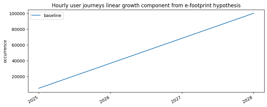
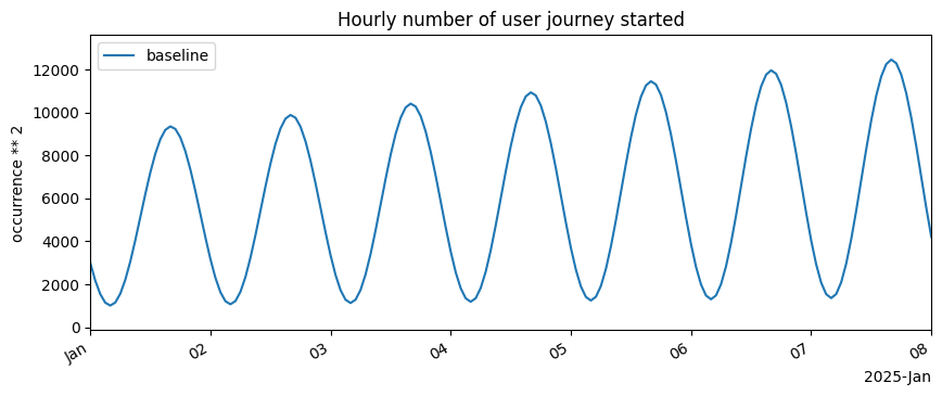
# Let’s build synthetic usage data by summing a linear growth with a sinusoidal fluctuation components, then adding daily variation
from datetime import datetime, timedelta

from efootprint.builders.time_builders import linear_growth_hourly_values

start_date = datetime.strptime("2025-01-01", "%Y-%m-%d")
timespan = 3 * u.year

linear_growth = linear_growth_hourly_values(timespan, start_value=5000, end_value=100000, start_date=start_date)
linear_growth.set_label("Hourly user journeys linear growth component")

linear_growth.plot()
from efootprint.builders.time_builders import sinusoidal_fluct_hourly_values

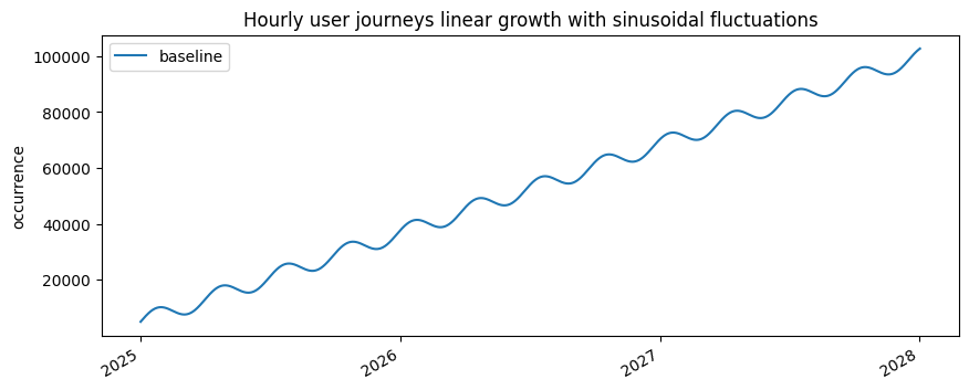
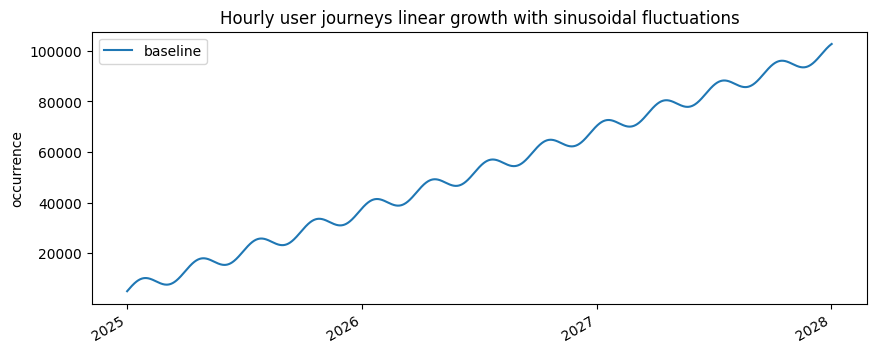
sinusoidal_fluct = sinusoidal_fluct_hourly_values(
    timespan, sin_fluct_amplitude=3000, sin_fluct_period_in_hours=3 * 30 * 24, start_date=start_date)

lin_growth_plus_sin_fluct = (linear_growth + sinusoidal_fluct).set_label("Hourly user journeys linear growth with sinusoidal fluctuations")

lin_growth_plus_sin_fluct.plot()
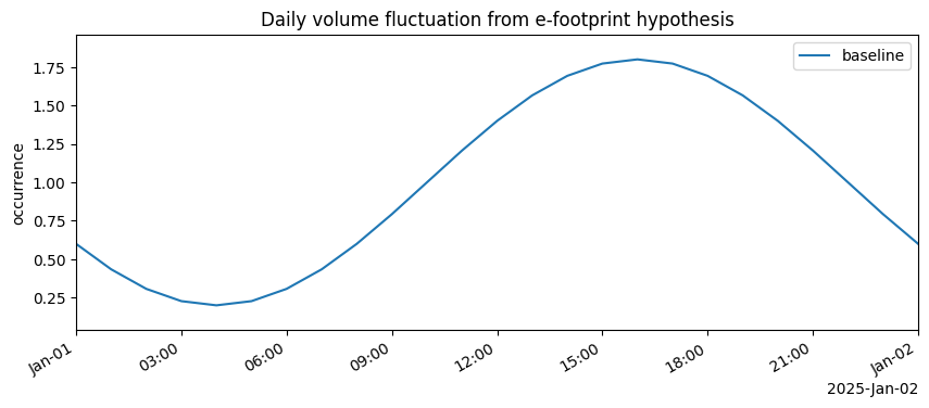
# Let’s add daily variations because people use the system less at night
from efootprint.builders.time_builders import daily_fluct_hourly_values

daily_fluct = daily_fluct_hourly_values(timespan, fluct_scale=0.8, hour_of_day_for_min_value=4, start_date=start_date)
daily_fluct.set_label("Daily volume fluctuation")

daily_fluct.plot(xlims=[start_date, start_date+timedelta(days=1)])
hourly_user_journey_starts = lin_growth_plus_sin_fluct * daily_fluct
hourly_user_journey_starts.set_label("Hourly number of user journey started")

hourly_user_journey_starts.plot(xlims=[start_date, start_date + timedelta(days=7)])
# Over 3 years the daily fluctuations color the area between daily min and max number of hourly user journeys
hourly_user_journey_starts.plot()
network = Network(
        "WIFI network",
        bandwidth_energy_intensity=SourceValue(0.05 * u("kWh/GB"), Sources.TRAFICOM_STUDY))

usage_pattern = UsagePattern(
    "Daily video streaming consumption",
    usage_journeys=[user_journey],
    devices=[Device.laptop()],
    network=network,
    country=Countries.FRANCE(),
    hourly_occurrences=hourly_user_journey_starts)

system = System("System", usage_patterns=[usage_pattern], edge_usage_patterns=[])
Results
Computed attributes
Now all calculated_attributes have been computed:
Server 7fb57669-696

name: server
carbon_footprint_manufacturing: 600 kg
power: 300 W
lifespan: 6 yr
fraction_of_usage_time: 1
server_type: autoscaling
idle_power: 50 W
ram: 128 GB ram
compute: 24 cpu core
power_usage_effectiveness: 1.2
average_carbon_intensity: 100 g/kWh
utilization_rate: 0.9
base_ram_consumption: 300 MB ram
base_compute_consumption: 2 cpu core
fixed_nb_of_instances: no value
storage: 57b7fe7a-4fe

calculated_attributes:
  raw_nb_of_instances: None
  nb_of_instances: None
  instances_energy: None
  instances_manufacturing_footprint: None
  use_footprint: None
  hour_by_hour_ram_need: None
  hour_by_hour_compute_need: None
  occupied_ram_per_instance: 2.3 GB ram
  occupied_compute_per_instance: 2 cpu core
  available_ram_per_instance: 113 GB ram
  available_compute_per_instance: 19.6 cpu core
  idle_use_footprint: None
  load_use_footprint: None
  fixed_nb_of_instances_validation: no value
  service_total_job_volumes: None
System footprint overview
Impact breakdown
e-footprint tracks impact repartition at each link in the object relationship chain, so you can have a complete understanding of where impact comes from both from a material and functional point of view.
from efootprint.utils.impact_repartition.sankey import ImpactRepartitionSankey

sankey = ImpactRepartitionSankey(
    system,
    # For each column in the Sankey diagram, nodes representing less than aggregation_threshold_percent% of total impact
    # are aggregated.
    aggregation_threshold_percent=1,
    # Allows for skipping certain object classes to simplify the diagram.
    skipped_impact_repartition_classes=None,
    # Specific columns have their own toggles.
    skip_phase_footprint_split=False, skip_object_category_footprint_split=False, skip_object_footprint_split=False,
    # It is also possible to exclude altogether certain object types from the total.
    excluded_object_types=None,
    # Also, it possible to filter on a specific life cycle phase.
    lifecycle_phase_filter=None,
    display_column_information=True,
    node_label_max_length=6
    )
sankey.figure(filename="Full impact repartition sankey.html", height=600, width=800, notebook=True)
2026-09-07 11:04:57,247 - INFO - Function build took 7.4 ms to execute.
2026-09-07 11:04:57,284 - INFO - Function figure took 44.8 ms to execute.
# Skipping certain classes (defined as strings or efootprint class objects) simplifies the view, for example
skipped_classes = ["System", "JobBase", "UsagePattern"]
sankey2 = ImpactRepartitionSankey(
    system,
    aggregation_threshold_percent=1,
    skipped_impact_repartition_classes=skipped_classes,
    skip_phase_footprint_split=False, skip_object_category_footprint_split=False,
    skip_object_footprint_split=False, excluded_object_types=None, lifecycle_phase_filter=None,
    display_column_information=True,
    node_label_max_length=6
    )
sankey2.figure(filename="Full impact repartition sankey skip jobs and usage patterns.html", height=600, width=800, notebook=True)
2026-09-07 11:04:57,289 - INFO - Function build took 0.6 ms to execute.
2026-09-07 11:04:57,318 - INFO - Function figure took 29.1 ms to execute.
# Now let’s exclude user devices and focus on usage phase
from efootprint.core.lifecycle_phases import LifeCyclePhases

sankey3 = ImpactRepartitionSankey(
    system,
    aggregation_threshold_percent=1,
    skipped_impact_repartition_classes=skipped_classes,
    skip_phase_footprint_split=False, skip_object_category_footprint_split=False,
    skip_object_footprint_split=False, excluded_object_types=["Device"], lifecycle_phase_filter=LifeCyclePhases.USE,
    display_column_information=True,
    node_label_max_length=6
    )
sankey3.figure(filename="Usage impact repartition sankey skip jobs and usage patterns exclude devices.html",
               height=400, width=800, notebook=True)
2026-09-07 11:04:57,322 - INFO - Function build took 0.4 ms to execute.
2026-09-07 11:04:57,345 - INFO - Function figure took 23.1 ms to execute.
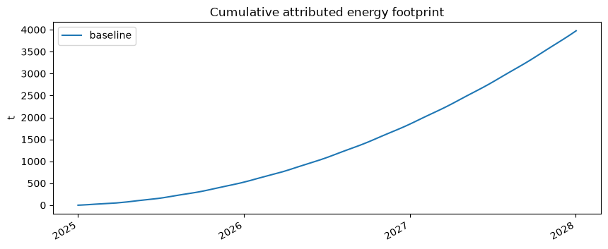
Besides the Sankey diagram, the attribution layer can be queried directly: attributed_footprint returns any object's share of the system footprint for a given life cycle phase.
from efootprint.core.attribution import attributed_footprint

# For example, the usage phase footprint attributed to the usage pattern
attributed_footprint(usage_pattern, LifeCyclePhases.USE).plot(cumsum=True)
Object relationships graph
Hover over a node to get the numerical values of its environmental and technical attributes. For simplifying the graph the Network and Hardware nodes are not shown.
from efootprint.utils.object_relationships_graphs import USAGE_PATTERN_VIEW_CLASSES_TO_IGNORE, INFRA_VIEW_CLASSES_TO_IGNORE

usage_pattern.object_relationship_graph_to_file("object_relationships_graph_up_view.html", width="800px", height="500px",
    classes_to_ignore=USAGE_PATTERN_VIEW_CLASSES_TO_IGNORE, notebook=True)
usage_pattern.object_relationship_graph_to_file("object_relationships_graph_infra_view.html", width="800px", height="500px",
    classes_to_ignore=INFRA_VIEW_CLASSES_TO_IGNORE, notebook=True)
usage_pattern.object_relationship_graph_to_file("object_relationships_graph_all_objects.html", width="800px", height="500px",
    classes_to_ignore=[], notebook=True)
Calculus graph
Any e-footprint calculation can generate its calculation graph for full auditability. Hover on a calculus node to display its formula and numeric value.
usage_pattern.devices[0].instances_manufacturing_footprint.calculus_graph_to_file(
    "device_population_fab_footprint_calculus_graph.html", width="800px", height="500px", notebook=True)
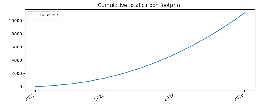
Plotting an object’s hourly and cumulated CO2 emissions
Analysing the impact of a change
Numeric input change
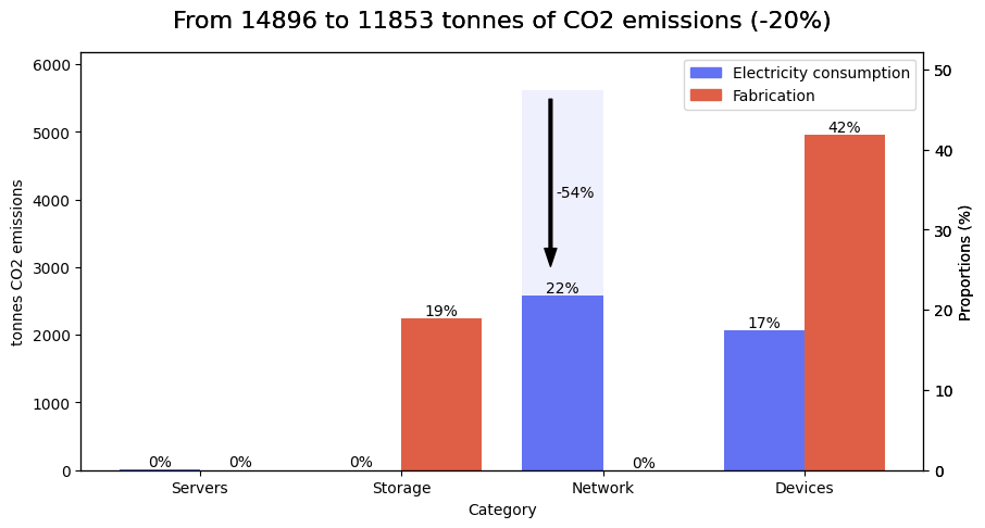
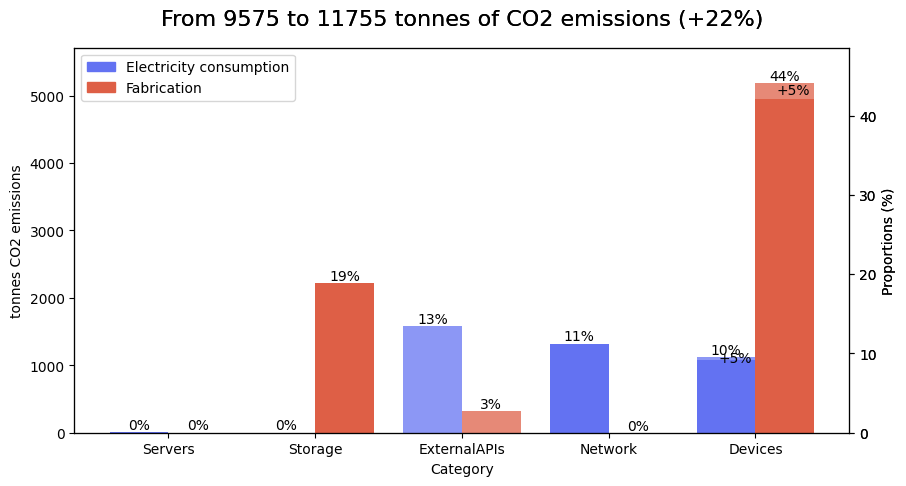
Any input change automatically triggers the computation of calculations that depend on the input. For example, let’s say that the average data download consumption of the streaming step decreased because of a change in default video quality. To analyse the impact of the change, let’s first save a copy of the system in its current state to compare against after the change:
# Snapshot the system in its current state to compare against after making changes
from efootprint.comparison.duplication import duplicate_system

initial_system = duplicate_system(system)
initial_system.name = "system before changes"

streaming_job.resolution = SourceObject("720p (1280 x 720)", Sources.USER_DATA)
2026-09-07 11:04:58,350 - INFO - 1 changes affected 22 reactive slots in 0.3 ms.
# System.compare_to returns a SystemComparison object exposing plots and structured diff data
comparison = initial_system.compare_to(system)
comparison.plot_decomposition("bandwith reduction.png")
System structure change
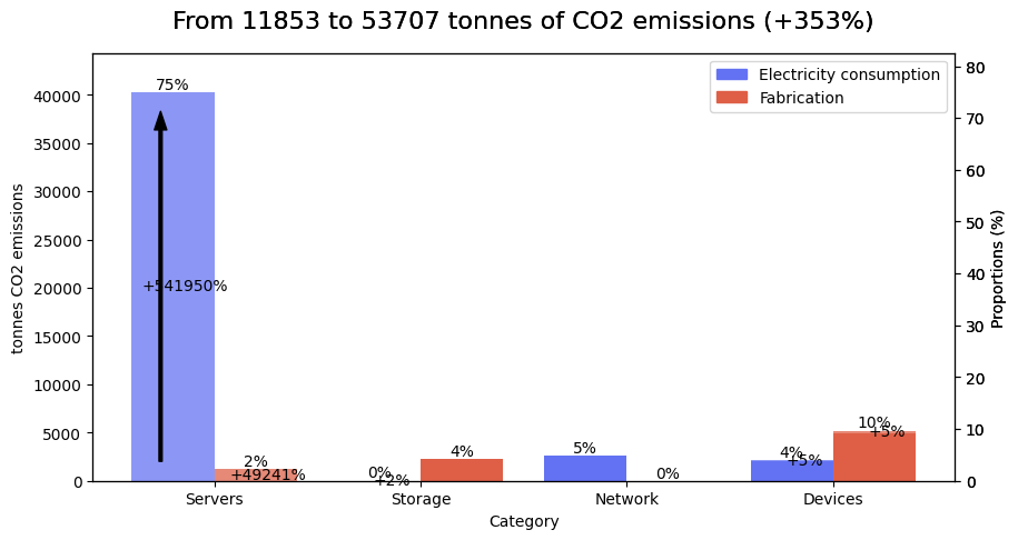
Now let’s make a more complex change, like adding a conversation with a generative AI chatbot before streaming the video. We will use e-footprint’s EcoLogitsGenAIExternalAPI object that runs EcoLogits’s LLM impact computations.
pre_llm_system = duplicate_system(system)
pre_llm_system.name = "system before LLM chat step"

from efootprint.builders.external_apis.ecologits.ecologits_external_api import EcoLogitsGenAIExternalAPI, EcoLogitsGenAIExternalAPIJob

genai_external_api = EcoLogitsGenAIExternalAPI(
    "Openai’s gpt-4o", provider=SourceObject("openai"), model_name=SourceObject("gpt-4o"))
genai_job = EcoLogitsGenAIExternalAPIJob("LLM API call", genai_external_api, output_token_count= SourceValue(1000 * u.dimensionless))

llm_chat_step = UsageJourneyStep(
    "Chat with LLM to select video", user_time_spent=SourceValue(1 * u.min, Sources.HYPOTHESIS),
    jobs=[genai_job])

# Adding the new step is simply a dict entry addition; the value is how many times the step occurs per journey.
user_journey.uj_steps[llm_chat_step] = SourceValue(1 * u.dimensionless)

usage_pattern.object_relationship_graph_to_file("object_relationships_graph_with_genai_infra_view.html", width="800px", height="500px",
    classes_to_ignore=INFRA_VIEW_CLASSES_TO_IGNORE, notebook=True)
2026-09-07 11:04:58,543 - INFO - 1 changes affected 69 reactive slots in 2.3 ms.
system.plot_footprints_by_category_and_object("System footprints with external gen AI API.html", notebook=True)
pre_llm_comparison = pre_llm_system.compare_to(system)
pre_llm_comparison.plot_decomposition("LLM chat addition.png")
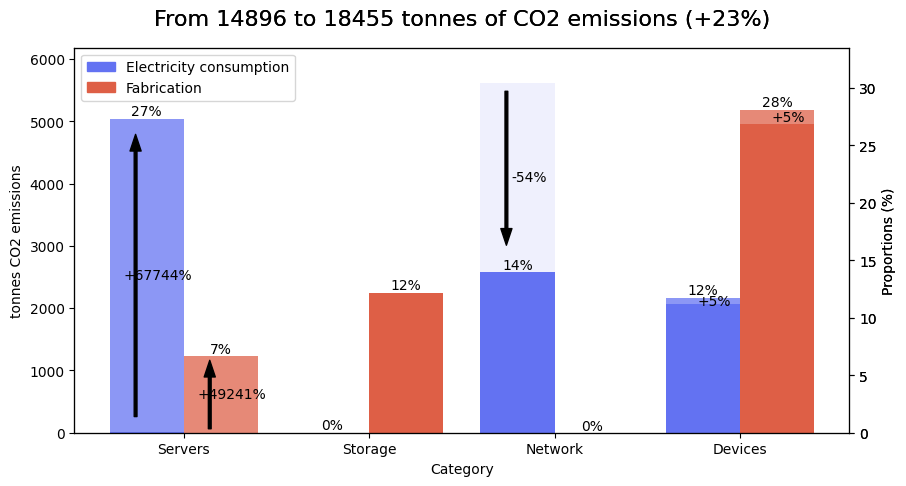
We can see that server use footprint has gone from almost zero to more than 1500 tonnes CO2-eq, and that the rest of the impact is quite negligible. Good to know to make informed decisions ! Of course the impact is very much dependent on assumptions. Let’s check out the external api server’s carbon intensity of electricity for example:
0.384 kg/kWh
# And let’s look at global impact repartition over both lifecycle phases
sankey4 = ImpactRepartitionSankey(
    system,
    aggregation_threshold_percent=1,
    skipped_impact_repartition_classes=skipped_classes,
    skip_phase_footprint_split=True, skip_object_category_footprint_split=False,
    skip_object_footprint_split=False, excluded_object_types=None, lifecycle_phase_filter=None,
    display_column_information=True,
    node_label_max_length=6
    )
sankey4.figure(filename="Full impact repartition sankey with external API skip jobs and usage patterns.html",
               height=600, width=800, notebook=True)
2026-09-07 11:04:58,894 - INFO - Function build took 9.5 ms to execute.
2026-09-07 11:04:58,920 - INFO - Function figure took 34.8 ms to execute.
Recap of all System changes
For richer side-by-side comparison of modeling scenarios with a graphical UI, check out the e-footprint interface.
comparison_from_start = initial_system.compare_to(system)
for diff in comparison_from_start.input_diff.changed:
    print(f"{diff.object_class} {diff.object_name_a} — {diff.attribute}: {diff.value_a} → {diff.value_b}")
comparison_from_start.plot_decomposition("All system diffs.png")
VideoStreamingJob streaming job — resolution: 1080p (1920 x 1080) → 720p (1280 x 720)

Reverting changes in batch
Changes can be applied (or reverted) in optimized batches with the ModelingUpdate object: recomputations run only once, after all changes have been applied.
# Let’s revert the system to its state before changes with a batch update
from efootprint.abstract_modeling_classes.modeling_update import ModelingUpdate

ModelingUpdate([
    [user_journey.uj_steps, {streaming_step: SourceValue(1 * u.dimensionless), upload_step: SourceValue(1 * u.dimensionless)}],
    [streaming_job.resolution, SourceObject("1080p (1920 x 1080)")]
])

system.plot_footprints_by_category_and_object("System footprints after reset.html", notebook=True)
2026-09-07 11:04:59,062 - INFO - 2 changes affected 100 reactive slots in 3.1 ms.
[Optional] Model edge devices
The above modeling reflects a centralized web logic: the input usage is a business input (typically, the number of visits on a website), and the infrastructure has to be sized to meet the demand. But there are cases where the usage is actually proportional to a number of devices, typically when trying to model the impact of selling digital devices, like servers, smartphones or video game consoles. In this case, e-footprint edge objects allow for the description of usage per device, and number of devices sold / produced over the modeling period.
Define the edge device
The EdgeStorage and EdgeDevice objects are similar to the Storage and Server objects, but simpler because they don’t have to include any autoscaling logic.
from efootprint.core.hardware.edge.edge_storage import EdgeStorage
from efootprint.builders.hardware.edge.edge_computer import EdgeComputer

edge_storage = EdgeStorage(
    "Edge SSD storage",
    carbon_footprint_manufacturing_per_storage_capacity=SourceValue(160 * u.kg / u.TB_stored),
    lifespan=SourceValue(6 * u.years),
    storage_capacity_per_unit=SourceValue(256 * u.GB_stored),
    base_storage_need=SourceValue(10 * u.GB_stored),
)

edge_computer = EdgeComputer(
    "Edge device",
    carbon_footprint_manufacturing=SourceValue(60 * u.kg),
    power=SourceValue(30 * u.W),
    lifespan=SourceValue(8 * u.year),
    idle_power=SourceValue(5 * u.W),
    ram=SourceValue(16 * u.GB_ram),
    compute=SourceValue(8 * u.cpu_core),
    base_ram_consumption=SourceValue(1 * u.GB_ram),
    base_compute_consumption=SourceValue(0.1 * u.cpu_core),
    storage=edge_storage
)
Define the edge usage journey with the processes that run on the edge device
The EdgeUsageJourney object groups reusable functionality that runs on edge devices. Deployment lifetime belongs to EdgeUsagePattern; each RecurrentEdgeProcess describes weekly compute, RAM, and storage demand starting at midnight on a Monday local time.
import numpy as np
from pint import Quantity

from efootprint.abstract_modeling_classes.source_objects import SourceRecurrentValues
from efootprint.builders.usage.edge.recurrent_edge_process import RecurrentEdgeProcess
from efootprint.core.usage.edge.edge_function import EdgeFunction
from efootprint.core.usage.edge.edge_usage_journey import EdgeUsageJourney

edge_process = RecurrentEdgeProcess(
    "Edge process",
    edge_device=edge_computer,
    recurrent_compute_needed=SourceRecurrentValues(
        Quantity(np.array([1] * 168, dtype=np.float32), u.cpu_core)), # 7 * 24 = 168 hours in the canonical week
    recurrent_ram_needed=SourceRecurrentValues(
        Quantity(np.array([2] * 168, dtype=np.float32), u.GB_ram)),
    recurrent_storage_needed=SourceRecurrentValues(
        Quantity(np.array([200] * 168, dtype=np.float32), u.kB_stored))
)

# edge functions are analogous to usage journey steps in that they allow the grouping of edge processes that serve the same purpose.
edge_function = EdgeFunction("Edge function", recurrent_edge_device_needs=[edge_process],
                             # Server needs will be presented in the next section
                             recurrent_server_needs=[])

edge_usage_journey = EdgeUsageJourney(
    "Edge usage journey",
    edge_functions=[edge_function]
)
Define the edge usage pattern
The EdgeUsagePattern object specifies the number of edge devices that are emitted in a given countrey across time, through its hourly_deployment_starts parameter. It could be for example the sales projection of a video game console seller. It is then linked to a System through System’s edge_usage_patterns parameter, just like web usage patterns are linked to a System through the usage_patterns parameter. That way, web and edge objects can coexist in the same simulation.
pre_edge_system = duplicate_system(system)
pre_edge_system.name = "system before edge devices"

from efootprint.builders.time_builders import create_hourly_usage_from_frequency
from efootprint.core.usage.edge.edge_usage_pattern import EdgeUsagePattern

edge_usage_pattern = EdgeUsagePattern(
    "Edge usage pattern",
    edge_usage_journeys=[edge_usage_journey],
    network=Network.wifi_network(),
    country=Countries.FRANCE(),
    hourly_deployment_starts=create_hourly_usage_from_frequency(
        timespan=5 * u.year, input_volume=10, frequency='weekly',
        active_days=[0, 1, 2, 3, 4, 5], hours=[9, 10, 11, 12, 15, 16, 17, 18, 19]),
    usage_span=SourceValue(6 * u.year)
)

system.edge_usage_patterns = [edge_usage_pattern]

system.plot_footprints_by_category_and_object("System with edge objects footprints.html", notebook=True)
2026-09-07 11:04:59,178 - INFO - 1 changes affected 2 reactive slots in 5.8 ms.
pre_edge_comparison = pre_edge_system.compare_to(system)
pre_edge_comparison.plot_decomposition("Add edge objects.png")

system.object_relationship_graph_to_file("system_with_edge_objects_graph_up_view.html", width="800px", height="500px",
    classes_to_ignore=USAGE_PATTERN_VIEW_CLASSES_TO_IGNORE, notebook=True)
system.object_relationship_graph_to_file("system_with_edge_objects_graph_infra_view.html", width="800px", height="500px",
    classes_to_ignore=INFRA_VIEW_CLASSES_TO_IGNORE, notebook=True)
[Optional] define requests made to web servers
RecurrentServerNeed objects allow for the description of recurrent requests made to a web server by an edge device. The recurrent volume will be multiplied by the number of edge device deployed, and will apply to the all the RecurrentServerNeed jobs (which can be used by other RecurrentServerNeeds, or even within WebUsageJourneySteps).
from efootprint.core.usage.edge.recurrent_server_need import RecurrentServerNeed

# Let’s create a new, simple server with default values
server = Server.from_defaults("New server", storage=Storage.from_defaults("New storage"))

# 2 jobs are triggered every hour, for each hour of the typical week
recurrent_volume = SourceRecurrentValues(np.array([2.0] * 168, dtype=np.float32) * u.occurrence)

job = Job.from_defaults("Job on new server", server=server)

server_need = RecurrentServerNeed(
            "Server need",
            edge_device=edge_computer,
            recurrent_volume_per_edge_device=recurrent_volume,
            jobs=[job])

edge_function.recurrent_server_needs.append(server_need)
2026-09-07 11:04:59,703 - INFO - 1 changes affected 18 reactive slots in 6.4 ms.
system.object_relationship_graph_to_file("system_with_edge_objects_graph_infra_view_with_server_job.html", width="800px", height="500px",
    classes_to_ignore=INFRA_VIEW_CLASSES_TO_IGNORE, notebook=True)